Electrical circuits form the backbone of modern technology, linking voltage, current, and resistance in predictable patterns. A study guide introduces core concepts, such as Ohm’s law, series‑parallel combinations, and basic schematic notation, empowering learners to analyze real‑world systems.!!??

Basic Components and Units

In a circuits study guide, the foundation lies in understanding the elementary elements that constitute any electrical network. Each component serves a distinct role, and their quantitative description relies on standardized units that enable clear communication and precise calculations.

• Voltage Source (V): Provides potential difference, measured in volts (V). Ideal sources maintain constant voltage.
• Current Source (I): Delivers a fixed current, measured in amperes (A). Ideal sources keep current constant.
• Resistor (R): Opposes current flow, quantified in ohms (Ω). Ohm’s law links voltage and current.
• Capacitor (C): Stores electric charge, quantified in farads (F). Capacitance determines charging rate.
• Inductor (L): Stores magnetic energy, quantified in henries (H). Inductance governs current change.
• Switch: Controls connectivity, toggling between open (infinite resistance) and closed (negligible resistance) states.
• Diode: Allows current in one direction, blocking reverse flow.
• Transistor (BJT or MOSFET): Acts as a switch or amplifier, controlling large currents with small input signals.

Power is is expressed in watts (W)and calculated as P = VI or P = I²R Energy, measured in joules (J) is the product of power and time.These units allow students to translate physical phenomena into equations

Ohm’s Law and Power Calculations

Ohm’s Law links voltage (V), current (I), and resistance (R) with V = IR. Power (P) is product of voltage and current, P = VI, or P = I²R. These equations let students compute energy use, design circuits, and analyze efficiency in real devices. Apply these formulas to solve and design circuits now

Voltage, Current, Resistance Relationships

Voltage, measured in volts, is the electric potential difference that drives charge carriers through a circuit. Current, expressed in amperes, represents the flow rate of electrons, while resistance, in ohms, quantifies how strongly a material opposes that flow. Ohm’s Law, V = IR, is the foundational equation linking these three quantities. It states that the voltage across a component equals the product of the current flowing through it and its resistance. This simple relationship allows engineers and students to predict how a change in one parameter will affect the others. For example, increasing resistance while keeping voltage constant will reduce current, whereas raising voltage with constant resistance will increase current proportionally. The law also implies that resistance can be expressed as R = V/I, and current as I = V/R, providing flexibility in solving circuit problems. In practical circuits, voltage sources such as batteries or generators provide the driving force, while resistive elements like resistors, incandescent filaments, or even the internal resistance of a power supply determine how much current flows. Power, the rate of energy transfer, is calculated as P = VI or P = I²R or P = V²/R, illustrating how voltage, current, and resistance jointly determine energy consumption or dissipation. Understanding these relationships is essential for designing safe, efficient, and functional electrical systems, from simple LED circuits to complex power distribution networks. All concepts are.

Series Circuit Analysis

In a series circuit, components share a single current path. The total resistance equals the sum of individual resistances, R_total = R1 + R2 + …, leading to voltage division across each element. Current remains constant, while voltage drops proportionally to each resistance. Simplifies analysis

Voltage and Resistance Distribution

When components are connected end‑to‑end, the same current flows through each resistor, and the total voltage supplied by the source is partitioned among them. The voltage drop across a resistor is proportional to its resistance, following Ohm’s law: V = I·R. Because the current I is identical for all series elements, the larger the resistance, the larger the voltage drop. The sum of all voltage drops equals the source voltage, ensuring energy conservation. Mathematically, V_total = ΣV_i = I·ΣR_i. This relationship allows engineers to predict how adding or removing a resistor changes the overall voltage distribution. For instance, inserting a high‑value resistor increases its share of the total voltage while reducing the voltage across the remaining components. Conversely, a low‑value resistor will drop only a small fraction of the total voltage. Practical applications include designing voltage dividers, where specific voltage levels are extracted by selecting appropriate resistor ratios. In such circuits, the ratio of the desired output voltage to the input voltage is V_out/V_in = R_selected/(R_total). Accurate calculation of voltage drops is essential for ensuring that each component receives the correct operating voltage, preventing over‑voltage damage or insufficient performance. By mastering voltage and resistance distribution in series circuits, students gain a foundational skill set for analyzing more complex networks and for troubleshooting real‑world electronic devices. In practice, engineers use simulation tools to verify voltage distribution before building prototypes, ensuring reliability and safety in devices ranging from simple LED circuits to complex power supplies. for all users andOK!!!!!!!!!

Parallel Circuit Analysis

In parallel networks, each branch shares the same voltage while currents divide inversely with resistance. The total current equals the sum of branch currents: I_total = V(1/R1 + 1/R2 + …). Equivalent resistance follows 1/R_eq = Σ(1/R_i). This rule underpins load.!!

Current and Resistance Distribution

In a parallel circuit, the voltage across each branch is the same, while the current divides inversely with resistance. Using Ohm’s law (I = V/R), branch currents are calculated once the common voltage is known. The total current supplied by the source equals the sum of all branch currents, and the equivalent resistance is found by the reciprocal rule: 1/R_eq = Σ(1/R_i). Adding more parallel branches lowers the overall resistance, increasing total current for a fixed source voltage. Engineers exploit this to design power distribution that keeps voltage stable across multiple loads. Current distribution is inversely proportional to resistance: a low‑resistance path draws more current, a high‑resistance path draws less. This principle guides component selection for safety and efficiency, preventing overheating in low‑resistance paths. Accurate analysis requires measuring each branch’s resistance and the source voltage, then applying the reciprocal rule to compute total current and verify each component operates within its limits. Mastering these concepts enables prediction of circuit behavior, fault diagnosis, and design optimization for reliability and performance.

In practice, designers often use a combination of series and parallel elements to tailor voltage and current levels to device requirements.By placing resistors, capacitors, and inductors, impedance can be controlled, ensuring that each load receives the appropriate power while maintaining system stability.

Kirchhoff’s Voltage and Current Laws

Kirchhoff’s rules extend Ohm’s law to networks.The Voltage Law states that the algebraic sum of potential differences around any closed loop equals zero, ensuring conservation. The Current Law dictates that the sum of currents entering a junction equals the sum leaving reflecting charge continuity

Application to Complex Networks

In complex electrical networks, Kirchhoff’s voltage and current laws become indispensable tools for systematic analysis. By selecting independent loops (mesh analysis) or junctions (nodal analysis), one can formulate a set of simultaneous algebraic equations that capture the behavior of every element. The mesh method assigns a loop current to each independent loop; the sum of voltage drops around that loop must equal the applied source voltage, yielding equations of the form ΣV = 0. Conversely, the nodal method assigns a node potential to each junction (except a reference ground) and applies the current law: ΣI entering a node equals ΣI leaving. This leads to equations of the form Σ(V_node – V_adjacent)/R = 0. Solving these linear systems—often with matrix techniques or computer algebra—provides the unknown currents and voltages throughout the network. Superposition, a direct consequence of linearity, allows complex circuits to be broken into simpler parts: each independent source is considered separately while others are replaced by their internal resistances, and the resulting responses are summed. For networks containing dependent sources, the analysis must incorporate the controlling variables, leading to augmented equations. Practical examples include power‑distribution grids, integrated‑circuit layouts, and multi‑stage amplifier designs, where accurate prediction of voltage drops and current paths is critical. Students can model circuits accurately, ensuring reliable operation across all scenarios and safety now. Practice regularly.

RC Circuit Behavior

An RC series circuit charges the capacitor following V(t)=V₀(1−e^(−t/RC)); The time constant τ=RC sets the charging speed; after 5τ the capacitor is nearly fully charged. During discharge V(t)=V₀e^(−t/RC) with the same τ, illustrating exponential decay. It is key timing.

Time Constant and Charge Curves

In an RC series network, the product of resistance (R) and capacitance (C) defines the time constant τ, expressed as τ = R × C. This single value governs how quickly the capacitor charges or discharges. During the charging phase, the voltage across the capacitor follows the exponential law V(t) = V₀ (1 – e^(–t/τ)), where V₀ is the source voltage. At t = τ, the capacitor reaches approximately 63.2 % of V₀; after 2τ it reaches about 86.5 %, after 3τ about 95 %, and after 5τ it is effectively fully charged. The discharge curve, starting from an initial voltage V₀, obeys V(t) = V₀ e^(–t/τ). The same τ appears in both equations, underscoring its role as the characteristic time scale of the system. Engineers use τ to design filters, timing circuits, and to predict transient behavior in power supplies and signal processing. By measuring the slope of the voltage curve on a logarithmic plot, one can extract τ experimentally. This method is fundamental in laboratory settings for verifying component values and ensuring proper circuit operation. The exponential nature of the curves also illustrates the memory effect of capacitors, as their voltage depends on the entire past current history, not just instantaneous conditions. Understanding τ and the associated charge curves is essential for mastering dynamic circuit analysis and for troubleshooting real‑world electronic devices that rely on precise timing and filtering characteristics. The exponential charging and discharging curves are symmetric in shape but differ in direction, reflecting the energy storage

Practical Applications of Circuits

Real‑world devices—from household appliances to automotive electronics—rely on series, parallel, and RC networks. Power supplies and signal filters use Ohm’s law and Kirchhoff’s rules to regulate voltage, current, and charge, ensuring reliable performance!.

Real-World Devices and Systems

In everyday life, circuits underpin countless devices that shape modern convenience and safety. Household appliances such as refrigerators, washing machines, and microwave ovens rely on regulated power supplies that use series and parallel resistor networks to maintain stable voltage and current, ensuring efficient operation and longevity. Lighting systems, from LED fixtures to incandescent bulbs, employ series‑parallel configurations to distribute current evenly across multiple elements, preventing flicker and extending bulb life. Automotive electronics illustrate the practical power of circuit theory: engine control units (ECUs) process sensor data through complex RC filters, while ignition coils use transformer principles to step up voltage for spark plugs. Communication devices, including smartphones and routers, depend on integrated circuits that integrate thousands of transistors, resistors, and capacitors into a single silicon chip, enabling high‑speed data transmission and signal processing. Industrial automation harnesses programmable logic controllers (PLCs) that execute control logic via discrete inputs and outputs, with safety interlocks implemented through series‑parallel resistor networks to detect fault conditions. Medical equipment such as MRI scanners and patient monitors incorporate precision voltage regulators and filtering circuits to deliver clean, noise‑free signals to sensitive detectors. Renewable energy systems, like solar inverters and wind turbine converters, use power electronics that convert DC to AC, employing series‑parallel arrangements of diodes and MOSFETs to manage current flow and protect against over‑voltage. In all these contexts, the fundamental principles of Ohm’s law, Kirchhoff’s rules, and RC time constants guide the design, ensuring reliability, efficiency, and user safety across diverse applications.!!!!!!!!!

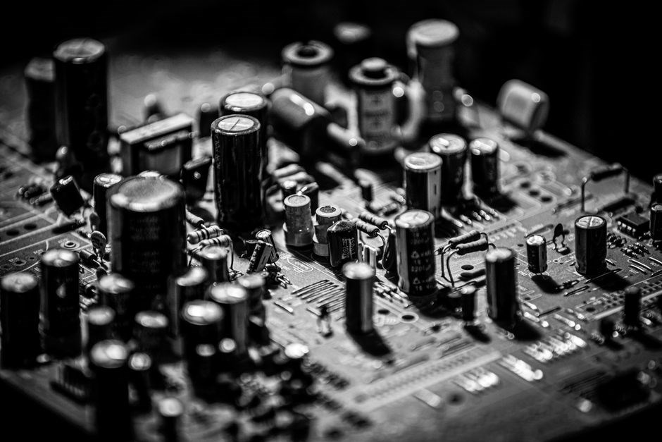
Troubleshooting and Safety Practices

Use a multimeter to check continuity, voltage, and resistance before touching wires. Verify power is off, label components, and follow lock‑out/tag‑out procedures. Inspect for overheating, frayed insulation, and connections to prevent shorts and fires.

Common Issues and Precautions

Common issues in circuit work range from simple miswired connections to subtle component failures. The most frequent problem is a short circuit caused by exposed leads or damaged insulation, which can trigger fuses or trip breakers. Over‑current conditions often result from using a resistor with a lower power rating than required, leading to overheating and eventual failure. Another typical error is incorrect polarity on polarized components such as electrolytic capacitors, which can cause rapid voltage spikes and component rupture. Loose solder joints or broken leads can introduce intermittent faults that are hardto detect during testing but may surface under load. Environmental factors such as humidity, temperature extremes, or dust infiltration can degrade contact surfaces and accelerate corrosion, especially in outdoor or industrial installations.

Voltage spikes from inductive loads can damage components; installing snubbers or varistors is recommended. Heat sinks should be attached to devices to avoid thermal runaway. Finally, always keep a spare set of components and a schematic diagram handy for replacementduring field repairs